
A defensible LTV, CAC and payback cohort model starts with money and customer behavior already observed. It then shows any continuation assumptions separately. Three months of contribution can support a three-month observation; it cannot establish a customer’s lifetime value or prove that the business can safely scale acquisition spending.
Build a cohort table, an acquisition-cost schedule and a cumulative contribution curve. You will need paid-customer start dates, invoices or collections, refunds, service costs, support records and acquisition spending. Decide whether the model measures accounting contribution or cash recovery. Keep that choice consistent throughout the calculation.
Define a customer, cohort and acquisition cost boundary
Choose the unit being acquired. A paid company account, individual subscriber, seat and free signup are different denominators. Define the event that starts the cohort, such as the first qualifying paid subscription, and preserve the cohort’s original membership when customers later cancel.
Stripe’s CAC guidance defines acquisition cost using sales and marketing costs relative to acquired paying customers and discusses timing and allocation complications. Use that as a framework, then document the business’s exact boundary. Do not divide a paid marketing bill by all free registrations.
Separate a narrowly defined campaign CAC from a fully loaded acquisition measure. The latter may include relevant sales labor, content, tools, agency costs and other acquisition work. An unpaid founder’s time can be valued separately for economic analysis, but it is not automatically a paid cash expense.
Match timing thoughtfully. A campaign paid in January may create customers in February. For a longer sales cycle, use an attribution or allocation method that fits the available evidence and state its limits. Merely dividing one calendar month’s spending by that month’s customers can produce a misleading comparison.
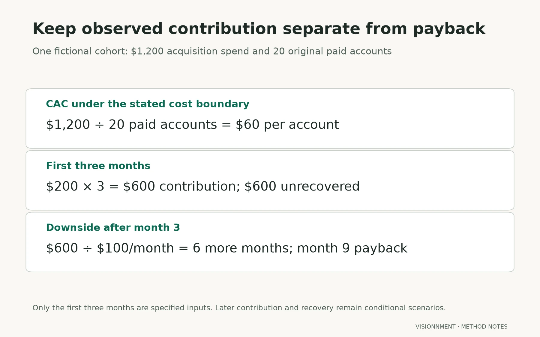
The hypothetical cohort in this guide spends $1,200 to acquire 20 paid accounts. Under that explicitly defined cost boundary, CAC is $60 per account. Additional omitted acquisition costs would change the fully loaded figure. This is a teaching case, not a measured campaign result.
Separate observed contribution from projected lifetime value
Create columns for cohort age, starting accounts, retained accounts, revenue or collections, direct costs and contribution. Compare cohorts at the same age. A six-month-old cohort has had more opportunity to contribute than one acquired last month.
ChartMogul’s cohort documentation explains grouping customers and examining behavior over time. Use the same principle in a spreadsheet if that is sufficient. Software-generated cohort tables still depend on accurate billing data and the chosen definitions.
Assume the hypothetical cohort contributes $200 in each of its first three observed months, after the stated direct costs. Observed contribution totals $600. Dividing that by the original 20 paid accounts gives $30 of observed contribution per acquired account over those three months.
| Cohort age | Status | Monthly contribution | Cumulative contribution |
|---|---|---|---|
| Month 1 | Observed hypothetical input | $200 | $200 |
| Month 2 | Observed hypothetical input | $200 | $400 |
| Month 3 | Observed hypothetical input | $200 | $600 |
| Months 4–6 | Continuation scenario only | $200 each | $1,200 by month 6 |
“Observed hypothetical input” means the case specifies those months for calculation; Visionnment did not operate or measure this cohort. In an actual model, replace those inputs with reconciled records and preserve the distinction between measured and forecast columns.
Stripe’s lifetime-value overview discusses methods that combine customer value and duration. Such estimates depend on assumptions about future behavior. A short, apparently stable history is not evidence that customers will remain indefinitely or continue contributing at the same rate.
Include gross margin, support and retention timing
State what the $200 contribution includes. For a useful operating analysis, identify the direct hosting, payment, service and support costs attributable to the cohort. Keep product development, central administration and other overhead visible elsewhere rather than implying contribution equals whole-business profit.
Distinguish gross margin from a more fully burdened contribution measure. If one channel acquires customers requiring more onboarding, its revenue can look attractive while its early contribution is weak. Allocate support consistently and avoid deducting the same cost both in CAC and again as service delivery.
Track retention at the level relevant to the product. Account retention, recurring revenue retention and usage are different measures. An account can remain active while reducing spend, or retain a paid contract while needing expensive support. Explain which change enters the model.
Preserve the timing of cash. Annual prepayments may recover acquisition cash early while leaving many months of service obligation. Monthly accounting revenue does not become monthly bank receipts simply because the model uses monthly columns. Build a separate cash schedule when prepayment materially changes the decision.
For refunds and disputes, link the adjustment to the relevant cohort and period. Do not improve a newer cohort’s apparent contribution by leaving its later reversals in an unallocated total. Equally, do not count a refund twice through both reduced revenue and a separate cost line.
Calculate cash payback using consistent periods
Define payback as the point when cumulative contribution under the stated boundary covers the acquisition investment. If the aim is cash payback, use actual cash timing for both acquisition outflow and customer contribution. If the table uses accrued contribution, label the result accordingly.
In the simplified hypothetical case, $1,200 divided by $200 monthly cohort contribution equals six months. The same result follows from $60 CAC per original account divided by $10 monthly contribution per original account. Both calculations require contribution to persist; only $600 has been specified for the first three months.
At month three, half of the defined acquisition cost remains unrecovered. State that plainly. “Six-month payback if contribution continues” is a scenario. “Payback achieved” would require evidence through the crossing point under the chosen cash or contribution definition.
Include the initial timing if costs are paid before the first customer receipt. A model beginning at the first paid month can omit the funding needed during a long acquisition cycle. Preserve negative or zero-contribution months rather than starting the clock when the picture becomes favorable.
If cumulative contribution never crosses the acquisition investment within the modeled horizon, report payback as unobserved or not reached in that scenario. Do not force a lifetime assumption until the spreadsheet produces an attractive answer.
Stress weak retention and rising acquisition cost
Vary one assumption at a time before combining downside cases. If the hypothetical cohort contributes only $100 monthly after month three, the remaining $600 requires another six months at that level. Payback would occur at month nine, assuming no further deterioration and no omitted costs.
If acquisition cost rises to $1,800 while contribution remains $200 monthly, simple modeled payback becomes nine months. This is another invented scenario, not a market forecast. The actual business could also see changing support cost, payment timing or customer mix.
Now combine a cost increase with weaker contribution and show the funding requirement. The purpose is to reveal which assumptions make the acquisition plan fragile. Do not present a collection of optimistic scenarios as a confidence interval or assign probabilities without evidence.
Investigate the mechanism behind a weak cohort. It may reflect customer fit, onboarding, product failure, payment issues or completion of an occasional-use task. A retention label alone does not identify the cause or the correct intervention. Keep the operating diagnosis separate from the arithmetic.
Retain zero-contribution and canceled accounts in the original cohort denominator. Removing them retrospectively can make the surviving customers appear to recover the acquisition investment faster than the original group actually did. Any survivor-only view needs a separate label and purpose.
Compare models without a universal ratio rule
Compare cohorts using the same cost boundary, maturity, currency and contribution definition. Segment where the business genuinely differs, such as channel, customer type or acquisition motion. Avoid drawing a causal conclusion from small or differently timed groups.
A ratio that looks attractive in one business can conceal slow cash recovery, concentrated customers or heavy ongoing service in another. Use the cohort model alongside reserves, operating capacity and customer evidence. It should inform a decision rather than replace diligence with a single target number.
For an acquisition, ask the seller to supply source records and explain the allocations. Reproduce material calculations before using projected lifetime value in underwriting. The small SaaS valuation guide connects retention and sustainable operating work with the broader valuation question.
Save a dated model containing observed months, scenario months, assumptions and unresolved data issues. State the next evidence checkpoint: for example, another fully reconciled cohort month or a corrected support allocation. The valuation methods guide is the next answer when the earnings basis is ready; the cohort table itself does not establish a sale price or future return.